As I continue to experiment with cheap software defined radios paired with open source software I find myself in awe of the amount of information passing silently all around us. More importantly, I’m in awe of what sharing that information with others has the potential to do. Learning and utilizing open source software are the first steps. Sharing with others the information it unlocks is the spark that ignites the fire.
A picture of the RF spectrum is worth a thousand words… perhaps.
This past week a local amateur radio group I belong to hosted their first 2-meter SSB talk-net. It went very well. Many members checked in and talked for almost an hour. Using my SDR and rtl_power, I decided to scan a small frequency range that included the frequency they would be using (144.230 MHz) for 4 hours. What I ended up capturing was pretty unique.
To the left is a processed image of the raw audio I was able to copy through my SDR and process in rtl_power. The scanned frequency range you see is 144.100 – 144.360 MHz. Again my frequency of interest was 144.230 MHz. I got a direct hit. I trimmed the image you see to hone in on two things.
1. A talk-net was occurring slightly off-frequency just before my group’s talk-net had begun.
2. Everything highlighted in the green box, top to bottom, represents 1 hour of elapsed time, the goal frequency, and a healthy received signal.
The areas that are yellow are received signals that surpassed the gain threshold set in the command line entry (which is explained below). The received transmissions from my group’s talk-net occupies the 144.230 MHz frequency range perfectly. What’s more, I sent this image to the founder of the group and here was his response.
“That’s awesome!! You can see the net on 144.240 then our net on 144.230!”
That’s rewarding. I sure as hell felt this way when I first saw it the image. The implications of this information are mind-boggling. It used to be that you had to listen to know what was going on and when. Now, I could run a scan for a week and tell you the most popular day on a frequency. I can tell you which FM radio stations never shut-up, or, which are the least chatty. Interestingly enough, I can tell you how often the BBQ joint near my place lets a customer know their order is ready (vibrating drink coaster). Likewise, I can tell you how many orders they fulfilled yesterday during their hours of operation. Fascinating.
But nothing happens unless I share the information.
With the group’s annual meeting coming up I hope to share more about what I’ve been able to uncover with ridiculously-affordable hardware and freely available open source software. The future is bright for this kind of exploration, and it’s already happening in pockets all around us. Give it a shot. You don’t even need to be a licensed ham radio amateur. Anyone can listen. Anyone.
Here are the commands I issued to initiate the SDR, produce the csv log file, and produce the heatmap image.
rtl_power -f 143.80:144.80:2k -p 20 -g 35 -i 1s -c 30% -e 4h 144_200-4h-1.csv
This command does the following:
-f (sets the frequency range: 143.800 – 144:800)
:2k (sets the bin size at 2k)
-p (corrects for errors in the SDR’s on-board crystal by +20 parts-per-million)
-g (sets gain at 35)
-i (sets write to log interval at 1 second)
-c (crops the data received by 30% – helps with larger csv files)
-e (sets the total elapsed time of the scan at 4 hours)
144_200-4h-1.csv is the file name of the log file that will be created and written to every second for 4 hours.
The end result was a 83.7 mb csv file. Once I had the file I then created a jpeg file from the data with the following command:
python heatmap.py 144_200-4h-1.csv 144_200-4h-1.jpg
The result has been trimmed and placed on the left of this blog post.